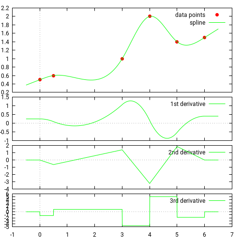
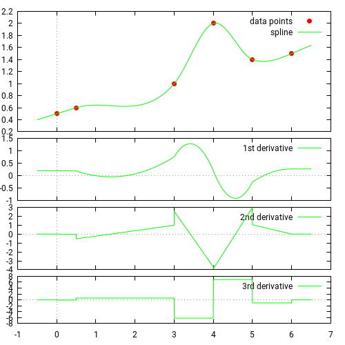
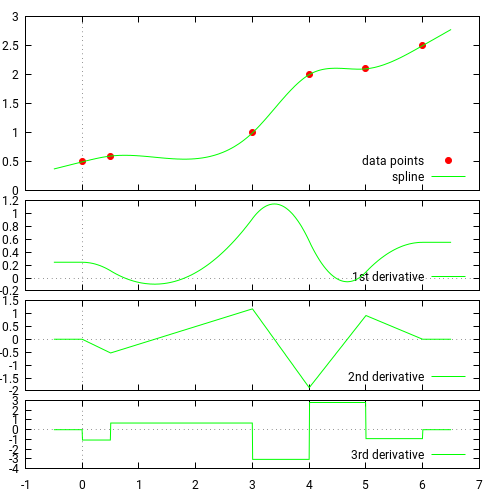
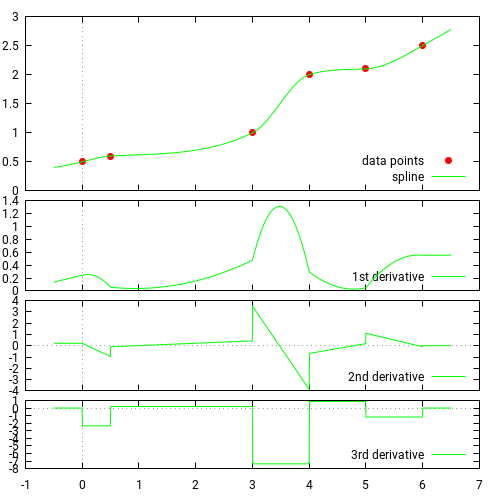
If input data is monotonic and the resulting spline is not monotonic,
it can be enforced via the make_monotonic() method.
Internally, this is achieved by reducing the slope on grid points adjacent to
non-monotonic segments (this breaks C2 and the resulting spline
is only C1).
cubic C2 spline
cubic monotonic spline
tk::spline s(X,Y,tk::spline::cspline); // or tk::spline s(X,Y);// alternatively
tk::spline s2;
s2.set_points(X,Y,tk::spline::cspline); // or s2.set_points(X,Y);
Left and right boundary conditions can be set via the constructor
or the set_boundary() method (must be called before
the set_points() method).
Periodic boundary conditions are currently not implemented.
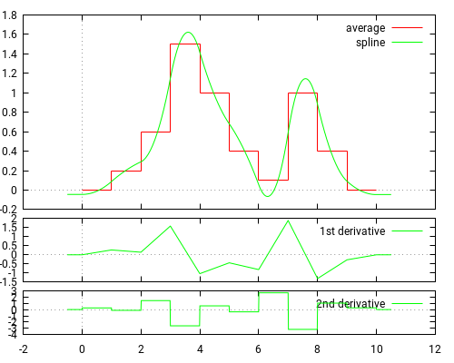
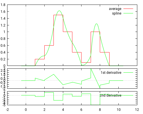
Mean preserving splines (average preserving, area preserving, mass preserving)
Sometimes one is given averages and needs to plot a smooth curve
which has equal averages, e.g. for histograms. Then the spline
does not interpolate points but has to satisfy the integral condition:
Luckily, this problem can be transformed so that any interpolating
spline can be used here. Define the integral function
$F(x) = \int_{x_0}^x f(t) \text{d}t$, then the above conditions are
equivalent to
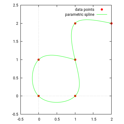
To connect arbitrary points in a 2D plane (or any n-D space) we
can simply introduce a "time" variable and treat every coordinate
as a function of time, i.e. every coordinate is interpolated via
a separate spline:
    // time proportional to distance, i.e. traverse the curve at constant speed
    T[0]=0.0;
    for(size_t i=1; i<T.size(); i++)
        T[i] = T[i-1] + sqrt( (X[i]-X[i-1])*(X[i]-X[i-1]) + (Y[i]-Y[i-1])*(Y[i]-Y[i-1]) );
    // setup splines for x and y coordinate
    tk::spline sx(T,X), sy(T,Y);
    ...
    double x = sx(t);
    double y = sy(t);
parametric spline
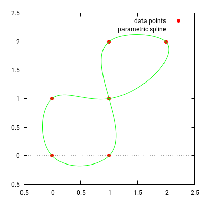
parametric closed spline
using natural boundary conditions, i.e. f''(a)=f''(b)=0
first and last point identical, i.e. x0=xn,
y0=yn
would need to use periodic boundary conditions, i.e. f'(a)=f'(b)
as a hack can also use natural boundary conditions and traverse
the closed curve a few times before drawing (done here)
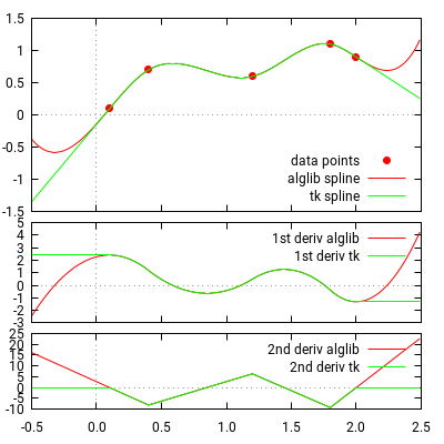
The result of this library is compared against
ALGLIB.
Interpolation
results are identical but extrapolation differs, as tk::spline
is designed to extrapolate linearly.
Source:
A simple benchmark shows that performance is comparable with
ALGLIB. The following
operations are measured:
Spline creation: calculate the coefficients of a spline given
input vectors X and Y,
Random access: evaluate spline(x), i.e. y-value of the spline at a random
point x,
Grid transform: given vectors X1,Y1, and a new vector X2, then we want
to calculate the corresponding Y2 vector, i.e. Y2[i]=spline(X2[i]).
Alglib outperforms here, because this operation can be implemented
more efficiently (TODO list).
The output "cycl" is the number of cpu cycles required for a single operation.
Below is just an outline. For more details see
spline.pdf.
$
\newcommand{\R}{\mathbb{R}}
\newcommand{\Co}{\mathrm{C}}
$
Input: a set of ordered $x, y$ coordinates
\begin{equation*}
\{(x_1,y_1),\dots,(x_n,y_n)\},\quad \text{with } x_1 < x_2 < \dots < x_n.
\end{equation*}
Output: a piecewise cubic function $f_i:[x_i,x_{i+1}]\to\R$,
\begin{equation}
f_i(x) = a_i + b_i (x-x_i) + c_i (x-x_i)^2 + d_i (x-x_i)^3.
\end{equation}
Define the space between $x$-points by $h_i:=x_{i+1}-x_i$.
Cubic C2 splines
Defined by
$f(x_i) = y_i$, i.e. $f$ interpolates all points,
$f\in\Co^2$, i.e. $f$ is twice continuously differentiable.
$f\in\Co^1$, i.e. $f$ is continuously differentiable,
$f'(x_i) = \delta_i$, i.e. derivatives are specified at each inner
point, e.g. by three point finite differences
\begin{equation*}
\delta_i=-\frac{h_i}{h_{i-1}(h_{i-1} + h_i)} y_{i-1}
+ \frac{h_i-h_{i-1}}{h_{i-1} h_i} y_i
+ \frac{h_{i-1}}{h_i(h_{i-1} + h_i)} y_{i+1}.
\end{equation*}
A sufficient (but not necessary) condition for monotinicity is
\begin{equation}
\sqrt{b_i^2+b_{i+1}^2} \leq 3 \frac{y_{i+1}-y_i}{h_i}.
\end{equation}
This can always be achieved by re-scaling $b_i$ and then re-calculating
$c_i$ and $d_i$ based on \eqref{eq:hermite_spline_coeffs}.
See also
Monotone piecewise cubic interpolation by Fritsch and Carlson.
Math symbols are rendered by MathJax
which requires JavaScript.