Numerical Simulation

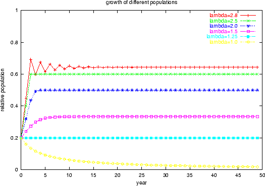
We can now examine the growth of some populations. First we are interested in the behaviour with low grow rates ( $1\leq\lambda_0\leq 2.8$). On figure 16 we can see the development over a time period of 50 years. The initial population is chosen as a fifth of the maximal population. Each population shows a stable growth. There is no visible change in the population after 50 years. Only the population with $\lambda_0=1$ will die out.

Figure 16: stable development of population

If we go up with the maximal growth rate to a value about $\lambda_0\approx 3$ (figure 17) the population is oscillating around a certain value.

Figure 17: development of population

For a even higher values we can observe a full range of different behaviours. In figures 18 to 21 some examples are shown.

Figure 18: Fluctuating between four different values

Figure 19: Fluctuating between a huge number of different values

Figure 20: Fluctuating in a more "chaotic" manner

Figure 21: Fluctuating between 3 values

Figure 22 shows the behaviour of populations after about 1000 years. The relative population after this time is given for different values of the maximal growth rate $\lambda _0$. In order to see if there is an fluctuation in the population after this time the values are plotted for the first 16 years after 1000 years.

Figure 22: Population after a long time depending on $\lambda _0$

This diagram shows:

max. growth rate	behaviour
$0\leq\lambda_0\leq 1$	population will die out
$1<\lambda_0\leq3$	population is stable after a sufficient long time, the relative population is exactly $1-\frac{1}{\lambda_0}$
$3<\lambda_0\leq 1+\sqrt6$	population fluctuates between two values
$1+\sqrt6<\lambda_0\leq...$	population fluctuates between four values
$\vdots$	$\vdots$
$\lambda_0\to 3.570...$	number of values the population fluctuates between goes up to $\infty$
$3.570...<\lambda_0<4$	many different types of behaviour including "chaotic" behaviour for certain values